doi: 10.56294/evk2025101

ORIGINAL

Application of a Methodological Framework for the Development of a HAZOP Study of a CSTR Reactor for the Production of Propylene Glycol from Propylene Oxide Using Process Simulation in Aspen HYSYS

Aplicación de un Framework Metodológico para la Elaboración del Estudio HAZOP de un Reactor CSTR de Producción de Propilenglicol a Partir de Óxido de Propileno Usando la Simulación del Proceso en Aspen HYSYS

Oswaldo A. Azuaje G¹, Andrés Rosales¹, Francisco Da Silva¹

¹Universidad Central de Venezuela, Facultad de Ingeniería, Escuela de Ingeniería Química. Caracas, Venezuela.

Cite as: Azuaje GOA, Rosales A, Da Silva F. Application of a Methodological Framework for the Development of a HAZOP Study of a CSTR Reactor for the Production of Propylene Glycol from Propylene Oxide Using Process Simulation in Aspen HYSYS. eVitroKhem. 2024; 3:101. https://doi.org/10.56294/evk2024101

Submitted: 05-06-2023                   Revised: 22-09-2023                   Accepted: 19-12-2023                 Published: 01-01-2024

Editor: Prof. Dr. Javier Gonzalez-Argote

ABSTRACT

HAZOP analysis is a systematic and structured method used to identify operational problems and potential hazards within a process. The methodology implemented, proposed in previous research, is based on the incorporation of process simulation to carry out a HAZOP study, through the construction of the process operating window and the establishment of deviations in the relevant process parameters. This methodology also includes a process layer analysis (LOPA), with special emphasis on the process design layers and the basic process control system. This research uses a CSTR reactor used in the production of propylene glycol through the hydrolysis reaction of propylene oxide as a case study, and was carried out using the commercial simulator Aspen HYSYS. For the initial operating conditions, a temperature of 91,63°C, a water conversion of 95 %, an outlet product flow of 10,29 mol/s, and a propylene glycol composition in the product of approximately 56 % were obtained in both cases. Using dynamic simulation, the deviations corresponding to the scenarios proposed were simulated, then the consequences observed were carefully analyzed, and preventive measures (known as safeguards) were proposed for each scenario. Finally, the study report was prepared based on the information obtained in the previous phase. The results obtained demonstrate that it is possible to effectively implement the methodology within the HYSYS simulator. In the short term, this methodology can be very useful as an initial stage of simulation-based process analysis, prior to the execution of a traditional HAZOP by a multidisciplinary group of experts in this method.

Keywords: Risk Analysis; Safety; HAZOP; CSTR Reactor; Propylene Glycol Production; Process Simulation; Aspen HYSYS.

RESUMEN

El análisis HAZOP es un método sistemático y estructurado usado para identificar los problemas de operatividad y los peligros potenciales dentro de un proceso. La metodología implementada, propuesta en una investigación previa, se fundamenta en la incorporación de la simulación de un proceso para llevar a cabo un estudio HAZOP, mediante la construcción de la ventana de operación del proceso y el establecimiento de las desviaciones en los parámetros relevantes del proceso. Esta metodología también incluye un análisis de capas de protección del proceso (LOPA), con especial énfasis en las capas del diseño del proceso y el sistema de control básico del proceso. En esta investigación se tiene como caso de estudio un reactor CSTR utilizado en la producción de propilenglicol por medio de la reacción de hidrólisis de óxido de propileno, y fue realizada usando el simulador comercial Aspen HYSYS. Para las condiciones iniciales de operación, se obtuvieron en ambos casos una temperatura igual a 91,63°C, una conversión del agua de 95 %, un flujo del producto de salida de 10,29 mol/s, y una composición de propilenglicol en el producto cercana al 56 %. Utilizando la simulación dinámica se simularon las desviaciones correspondientes a los escenarios planteados, después se analizaron detenidamente las consecuencias observadas y se propusieron medidas preventivas (conocidas como salvaguardas) para cada escenario. Finalmente, se procedió a elaborar el reporte del estudio realizado, a partir de la información obtenida en la fase anterior. Gracias a los resultados obtenidos se ha demostrado que es posible poner en práctica la metodología dentro del simulador HYSYS de manera efectiva. A corto plazo esta metodología puede ser de gran utilidad como una etapa inicial de análisis de un proceso basada en simulación, previa a la ejecución de un HAZOP tradicional por un grupo multidisciplinario de expertos en dicho método.

Palabras clave: Análisis de Riesgos; Seguridad; HAZOP; Reactor CSTR; Producción de Propilenglicol; Simulación de Procesos; Aspen HYSYS.

INTRODUCTION

This focuses on the application of a methodological framework for conducting a HAZOP study of a CSTR reactor used in the production of propylene glycol from propylene oxide. This framework includes the use of process simulation in risk analysis.^(1,2,3,4) The purpose of the study is to identify the risks inherent in this process and propose preventive safety measures for each of them to ensure that the reactor operates efficiently and safely.^(5,6,7)

In the future, this work is expected to contribute to the safety field by implementing an innovative methodology that improves the original HAZOP risk analysis method.^(8,9,10,11) This methodology seeks to optimize the identification of hazards in a process and to promote the integration of advanced technologies, such as simulation-based software tools, with traditional risk analysis methods.^(12,13,14) Dynamic simulations are of great value during the process design stage and for understanding potential failures that may arise during operations.^(15,16) For this reason, in the short term, the proposed methodology could be established as a necessary preliminary step before carrying out traditional HAZOP to minimize execution time and increase confidence in the results. In this way, it is expected that industrial facilities will not only be safer but also more efficient, thus contributing to the sustainability and operational continuity of processes.

Objective

To apply a methodological framework for the HAZOP study of a CSTR reactor used in the propylene glycol production process, using process simulation in Aspen HYSYS.

METHOD

Create a steady-state model of the reactor simulation and adjust it to generate the equipment operating window

The design and optimization of a chemical process involve studying it as it is carried out in both steady state and dynamic mode. Steady-state models allow steady-state mass and energy balances to be performed to evaluate different scenarios in a process. This simulation is also frequently used to prevent potential operating problems, as it allows the effect of changes in operating conditions on other process variables to be predicted. This way, more favorable control points can be established when performing the dynamic simulation. For all the reasons mentioned above, at this point, we propose performing the reactor simulation in a steady state since it will be used to construct the reactor's operating window and for the subsequent generation of the bifurcation diagram. Using steady-state simulation, it is possible to obtain the solutions for the different steady states and the ignition and extinction points.

Create a dynamic model of the reactor simulation and adapt it to simulate the events proposed in the HAZOP

This objective involves performing a dynamic simulation of the reactor. This simulation is critical, as chemical plants are never in a steady state. Using dynamic simulation, it can be confirmed that the plant can achieve the desired product safely and efficiently. Dynamic simulation is used to design and test various control strategies before choosing one suitable for implementation in each case.

It also allows for the analysis of start-up and shutdown procedures (scheduled and emergency), fluctuations in process parameters, the dynamic response of the system to unexpected disturbances or device failures, and the effects of control system intervention on the process. Analysis of the dynamic model can provide critical information for improving the steady-state model by identifying specific areas of the process that have difficulty achieving the objectives set during the steady-state analysis. In the case of this work, dynamic simulation will be used to support the construction of the reactor operating window and the bifurcation diagram since steady-state simulation does not allow the location of Hopf bifurcation points or the observation of the behavior of stable, oscillating, and unstable zones.

Construct the reactor operating window considering the multiplicity of steady states (stable, oscillating, and unstable)

The operating window of a piece of equipment comprises the parameters under which that equipment can operate without failure. This objective involves creating the operating window for the CSTR reactor studied, which is necessary to perform other process analyses later. In the case of a CSTR reactor with an exothermic reaction, it is essential to consider the existence of multiple steady states, as this is a crucial characteristic in studying its operation.

Establish the HAZOP deviations for the scenarios to be studied

The next step in the proposed methodological framework is to establish the deviations that will be used to evaluate the HAZOP scenarios subsequently. In a standard HAZOP study, deviations in all relevant process parameters are generated and investigated. However, in this HAZOP study, only the propylene oxide feed flow was considered a representative parameter to demonstrate the methodology's effectiveness. The events related to the disturbances to be simulated will be proposed using the contents of the primary bibliographic source supporting this work as a reference.⁽¹⁾

Unlike the traditional HAZOP procedure, this methodology uses the reactor operating window to determine the size of deviations that lead the reactor from one steady state to another. For this study, several simulation runs will be performed, introducing increases and decreases in the propylene oxide flow, varying the parameter from 0 to 30 mol/s, and considering the other relevant elements contained in the operating window within the analysis, such as stable and oscillating zones, ignition and extinction points, and Hopf bifurcation points.

Simulate the HAZOP events by analyzing the deviations, consequences, and safeguards

The work proposed in this objective consists of simulating the scenarios proposed in the reactor HAZOP using dynamic simulation while analyzing each of them during each run. This analysis consists of introducing the deviations of each scenario into the simulation and observing their consequences on the system's behavior. The study will be carried out in two stages: one open loop and one closed loop. The open loop stage seeks to show the consequences of the deviations if the controllers' corrective actions were not present during the equipment operation. In contrast, the closed loop stage evaluates whether the safeguards can effectively counteract these consequences.

At this point, the work proposed in this objective is precisely the analysis of the process protection layers. In the open-loop simulation stage, the layer corresponding to the process design is evaluated, while in the closed-loop simulation stage, the layer associated with the basic process control system is studied.

Generate the reactor bifurcation diagram to provide a graph representing the deviations and consequences of the transient events considered in the HAZOP

The Hopf bifurcation diagram, already discussed in the previous chapter, is very useful for performing reactor safety analysis because it allows various elements related to equipment operation to be visualized. Among these, it is important to highlight the effects of disturbances and controller actions, as well as stable, oscillating, and unstable zones. Using the bifurcation diagram, it is easier to observe the consequences of disturbances and the operational risks associated with the operation of the equipment.

Prepare the HAZOP study table for the reactor using the information obtained from the equipment simulation.

Finally, the last step of this work is to create the typical HAZOP study table for the reactor using the information from the tests done in the previous sections.

RESULTS AND DISCUSSION

Results of the steady-state simulation

This section created a model of the reactor simulation in a steady state. In general, as indicated in the literature consulted, a CSTR reactor with a cooling system produces propylene glycol from propylene oxide since the hydrolysis reaction is exothermic, and heat must be removed from the equipment to keep it operating at a safe temperature. As indicated in section II.2.1, the data selected for the simulation are the same as those for the case studied in the primary bibliographic source for this work.⁽¹⁾ These data are presented in the following table.

Table 1. Simulation data in steady state
Reagent inlet temperature (°C)	26
Propylene oxide flow (mol/s)	10
Water flow (mol/s)	6
Reactor volume (m3)	4
Liquid volume level in the reactor (%)	50
System pressure (kPa)	2000
Kinetic data
A(m^3/kmol·s)	9,6· 10^7
E(J/mol)	75362
Heat of reaction (J/mol)	-90000
Reaction order of the oxide (adím)	1
Water reaction order (adim)	1
Cooling system data
UA (W/°C)	7000
Cooling water flow (mol/s)	150
Cooling water inlet temperature (°C)	15
Water CP (kJ/kmol · °C)	75

It is important to note that because the simulator in this state does not allow direct use of the energy flow coupled to the reactor, additional tools were necessary to overcome this inconvenience. The tools used were an adjuster (Adjust) and a spreadsheet (Spreadsheet). These were used to adjust the reactor temperature so that its value changed and to calculate the heat exchanged using the spreadsheet until the estimated value matched the value calculated internally by the reactor. Using these tools ensures that the reactor will operate at a temperature at which the heat generated can be adapted to the capacity of the cooling water to remove heat from the system, as this is limited. The steady-state simulation diagram is shown in the following figure:

Figure 1. Diagram of the steady-state simulation

Once the proper functioning of the new tools connected to the reactor had been verified, the results corresponding to the base case study were generated. These results are shown in the following table:

Table 2. Results of the steady-state simulation
Reactor temperature (°C)	91,63
Water conversion (%)	95,24
Conversion of oxide (%)	57,14
Molar flow of the product (mol/s)	10,29
Molar fraction of propylene glycolin the product stream (adim)	0,555
Molar fraction of propylene oxide in the product stream (adim)	0,417
Molar fraction of water in theproduct stream (adim)	0,028
Vent outlet flow (mol/s)	0,00
Heat transferred (kJ/h)	-1,438·10^6
Cooling water outlet temperature (°C)	50,50

Generally, the results obtained are acceptable because water conversion was greater than 92 %, which meets the expected performance condition for the reaction indicated in the primary reference for this research.⁽¹⁾ Although the exact temperature of 86°C reported was not obtained, these results are still valid since the data used were verified many times during the simulation model's development. Therefore, the difference in temperatures could be attributed to the difference in the values used for the reaction heat (value set by the simulator, with no possibility of making changes) or to the use of a different thermodynamic model in both studies. These are the only data for which it was impossible to verify an exact match between the values used and those reported in the bibliographic reference. Despite this fact, further information supporting the results' validity will be presented below.

Results of the simulation in dynamic mode

Once the steady-state simulation stage was completed, the reactor simulation model was created in dynamic mode, considering that this model must be adaptable to simulate the different deviations to be analyzed in the HAZOP. The proper functioning of the dynamic simulation is critical in this research since the analyses to be performed later depend primarily on its ability to generate reliable results. At this point, it is essential to note that due to possible differences in the heat transfer equations used by the user and the simulator internally, it was necessary to adjust to obtain the desired results (i.e., that the results of the dynamic simulation matched those obtained through the steady-state simulation). This adjustment changed the heat transfer coefficient from 7000 W/°C to 9690 W/°C, the latter being obtained by trial and error within the simulation. The table below shows the data from the simulation in dynamic mode, followed by a diagram of the process.

Table 3. Dynamic simulation data
Reagent inlet temperature (°C)	26
Set point of the propylene oxide flow controller (mol/s)	10
Water flow controller set point (mol/s)	6
Reactor volume (m3)	4
Temperature controller set point (°C)	91,63
Liquid level controller set point (%)	50
System pressure (kPa)	2000
Kinetic data
A(m^3/kmol · s)	9,6· 10^7
E(J/mol)	75362
Heat of reaction (J/mol)	-90000
Reaction order of the oxide (adím)	1
Water reaction order (adim)	1
Cooling system data
UA (W/°C)	9690
Cooling water flow (mol/s)	150
Cooling water inlet temperature (°C)	15
Water CP (kJ/kmol · °C)	75

Figure 2. Diagram of the simulation in dynamic mode

The main difference between the two simulations is that controllers must be incorporated in dynamic mode for the most relevant variables related to reactor operation. As with the steady-state model, once the controllers had been assembled and configured in the simulation, the results of the base case study were calculated to verify their proper functioning. The corresponding results are presented in the following table.

Table 4. Results of the dynamic simulation
Reactor temperature (°C)	91,63
Water conversion (%)	95,18
Oxide conversion (%)	57,11
Molar product flow (mol/s)	10,29
Molar fraction of propylene glycolin the product stream (adim)	0,555
Molar fraction of propylene oxide in the product stream (adim)	0,417
Molar fraction of water in theproduct stream (adim)	0,028
Vent outlet flow (mol/s)	1·10-12
Heat transferred (kJ/h)	-1,436·10^6
Cooling water outlet temperature(°C)	50,46

These results confirm the proper functioning of the model created, as they are almost identical to the results obtained through stationary simulation. A comparative table of the results was prepared to appreciate better the similarities between the values obtained through both simulations, considering the differences and calculating the relative errors associated with each variable. The table containing this information is presented below:

Table 5. Comparative table of the results of the stationary simulation and the dynamic simulation
Process variable	Stationary simulation	Dynamic simulation	Difference	Relative error (%)
Reactor temperatura (°C)	91,63	91,63	0	0,00
Water conversion (%)	95,24	95,18	-0,06	0,06
Oxide conversion (%)	57,14	57,11	-0,03	0,05
Molar flow rate of the product(mol/s)	10,29	10,29	0	0,00
Molar fraction of propylene glycol in the product stream(adim)	0,555	0,555	0	0,00
Molar fraction of propylene oxide in the product stream(adim)	0,417	0,417	0	0,00
Molar fraction of waterin the product stream (adim)	0,028	0,028	0	0,00
Heat transferred (kJ/h)	-1,438· 10^6	-1,436· 10^6	2000	0,14
Cooling water outlet temperature (°C)	50,50	50,46	-0,04	0,08

Looking at the comparative table, the remarkable coincidence between the results of the steady-state simulation and the dynamic mode simulation stands out. The margins of error obtained are minimal.

Results of the construction of the reactor operating window

The first step in this stage consisted of generating several reactor temperature curves as a function of the propylene oxide flow for different cooling water flows, using steady-state simulation. The family of curves generated can be seen in the figure below:

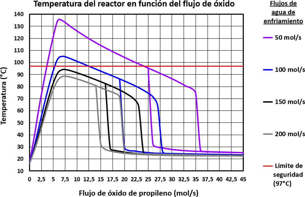
Figure 3. Steady-state solution family diagram: reactor temperature as a function of propylene oxide flow, for different cooling water flow rates

The generated curves show the expected behavior; they are shaped like an inverted “S” and clearly show the upper and lower steady states, as well as the ignition and extinction points. The graph also shows how the reactor temperature decreases as the cooling water flow increases.

For the next step, a comparison was made between the graph obtained and a new graph generated with data extracted from the previous work that supports this research,⁽¹⁾ as well as another previous publication by the same group of researchers, also related to this topic.⁽²⁾ The image now presented was designed to make this comparison:

Figure 4. Comparative image of the results obtained for the family of steady-state solutions, with respect to the reference graph

A substantial similarity between the two can be observed when comparing this graph with the one generated for reference. The similarity between the curves for cooling water flows of 100 mol/s and 150 mol/s is remarkable; in both graphs, the 100 mol/s curve exceeds the red line that defines the safety limit established for temperature, while the black curve representing the 150 mol/s flow is already below this limit and can be considered a safer flow option for operating the reactor. The same is true for the 200 mol/s curve, which was smaller than the 150 mol/s curve, and the same trend can be seen in the reference curve. In the case of the remaining curves, as the flows are not the same, the only comparable factor is the size of the curves. It can be seen that the 50 mol/s curve was larger than the 100 mol/s curve, and this also happens with the 80 mol/s curve in the reference graph. In summary, as the similarity between the two results is remarkable, the trend obtained is as expected and acceptable.

From the curves generated, one must be selected to use the corresponding cooling water flow for the simulation runs. In order to subsequently establish a better comparison between the results of this work and those of the reference cited in the next stage, it was decided to maintain the same cooling water flow of 150 mol/s.

The curve corresponding to this cooling water flow is shown individually below:

Figure 5. Reactor temperature curve as a function of propylene oxide flow, for the selected cooling water flow of 150 mol/s

Finally, to complete the construction of the equipment's operating window, it was necessary to run dynamic simulations varying the propylene oxide flow since, in steady-state simulation, it is impossible to identify stable, unstable, or oscillating operating points. The final result of the construction of the reactor's operating window is shown in the following figure:

Figure 6. Reactor operating window for selected cooling water flow of 150 mol/s

At this point, explaining the procedure used to identify the different operating zones is vitally important. The bifurcation points were found by running several dynamic simulations using a function called “ramp,” which allows a variable to be changed as a function of time, specifying a rate of change. A bifurcation point (or change in the operating zone) can be identified when the system variables suddenly oscillate after remaining stable for a specific period, as the ramp slowly changes the flow of propylene oxide. Following this procedure, it was possible to identify the stable and oscillating zones by observing the behavior of the temperature and other variables during the runs. This procedure is described in detail below.

Starting the runs at the selected normal operating point of 10 mol/s and using the ramp to decrease the oxide flow, a bifurcation point could be located for an oxide flow of 6 mol/s as the temperature and other monitored variables began to fluctuate sharply at this point. It can be stated with certainty that if the oxide flow decreased below this value, the reactor would enter an oscillating zone. Subsequently, in new runs using the ramp to increase the oxide flow, it was possible to verify the location of the extinction point obtained through the steady-state simulation for a flow of 23 mol/s. The stability of the reactor in this range was also verified during the same runs. New runs were also carried out to determine the system's behavior in the lower steady-state zone, achieving oscillating behavior, even when changing the reactor start point to another oxide flow in some runs. Due to the oscillating behavior in the indicated zone, it was impossible to verify the location of the ignition point; during the runs, the sudden temperature rise that usually occurs in this particular case was never observed. All runs in this test series were performed with the temperature controller operating in an open loop (manual mode), and the results presented in the following section effectively demonstrate that the behavior indicated in the operating window for each zone is correct. In the case of unstable steady states, it should be noted that these points were not located during the simulation runs but were represented (using a straight line) knowing that they lie between the upper and lower steady states and joining the ignition and extinction points, as indicated in the literature consulted. Finally, in the operational window constructed, it can be seen that the reactor has a single stable zone located at the top between the oxide flows of 6 mol/s and 23 mol/s (the extinction point). There are also two oscillating zones; one for oxide flow values less than 6 mol/s and the other coinciding with the lower steady-state zone.

Once the operating window was constructed, the result was compared with the corresponding reference. The image designed for comparison purposes at this point is shown below.

Figure 7. Comparative image of the result obtained for the reactor operating window, with respect to the reference graph

When comparing the graphs, it is clear that both show very similar patterns in the distribution of temperatures as a function of propylene oxide flow, despite some differences in the different steady states represented in each of them. Two differences between the graphs can be considered important. The most notable difference is that the reference shows the lower steady states as a stable zone, while oscillating behavior was observed in that zone in this study. The second difference is found in the curve of the upper steady states, just above the unstable states. The reference graph indicates that these points are oscillating states, unlike the results obtained in this study, where a stable zone was found for these points. Likewise, a minimal interval in the reference graph shows a stable zone. However, this is less relevant since both graphs practically oscillate throughout this interval (from 0 to the bifurcation point near the operating point). Despite the differences between the graphs, the general trend observed in both is consistent, which provides a solid basis for asserting that the results obtained for the reactor's operating window in this investigation are credible.

Establishment of HAZOP deviations

Before running the dynamic simulation, the deviations to be studied at this investigation stage were established. The selection was made so that these deviations would demonstrate the reactor's behavior in the different zones found during the construction of the operating window. In addition to the deviations, the reasons for their selection and the initiating causes that could cause the equipment to exceed its safe operating limits are presented. It is important to note that this study did not perform a rigorous analysis to identify the initiating causes of possible hazardous scenarios within the simulation. Although previous studies include this analysis in their methodology,⁽³⁾ this study has limited itself to taking the causes from the primary reference that served as the basis for this work⁽¹⁾ and presenting them in this section. The following table contains the corresponding information:

Table 6. Deviations established to be evaluated in the HAZOP study
Setting	Keyword	Established deviation	Final value of the oxide flow (mol/s)	Selection criteria	Possible causes^(1)
A	More	Propylene oxide flow (+30 %)	13	Follow the procedure for the main reference Evaluate a point within the stable zone	Propylene oxide feed valve failure
B	More	Propylene oxide flow (+60 %)	16	Evaluate a point within the stable zone	Propylene oxide feed valve failure
C	More	Propylene oxide flow (+150 %)	25	Evaluate a point within the oscillating zone, passing the extinction point	Propylene oxide feed valve failure
D	Minus	Propylene oxide flow (-40 %)	6	Evaluate a point within the oscillating zone for low oxide flows.	Pump failure

The figure below shows the points reached by the propylene oxide flow in each zone within the reactor operating window when the deviations indicated in the table above are introduced. The points are identified by circles, each containing the letter corresponding to each scenario.

Figure 8. Identification of points reached by the propylene oxide flow with the established deviations for each HAZOP scenario

Results of the HAZOP event simulation

Different dynamic simulation runs were carried out to analyze each of the possible deviation scenarios proposed by HAZOP to meet this objective. The runs consisted of starting and maintaining the reactor without disturbances and stopping the integrator after 2 hours. At that point, the deviations were manually introduced, and the integrator was allowed to run again until the 10 hours were completed, strictly following the procedure outlined in the primary reference for this work.⁽¹⁾ Similarly, following this procedure, the simulation was initially run in an open loop (turning off the controllers) and then in a closed loop (turning on the controllers).

Open loop system analysis

This section presents the results of the system operating in an open loop. As indicated in the previous section, four possible scenarios were considered for the HAZOP study: Scenario A assumes a 30 % increase in propylene oxide flow, scenario B a 60 % increase in oxide flow, scenario C a 150 % increase in flow, and finally, scenario D assumes a 40 % decrease in flow. The red curve represents the reactor temperature, and the propylene oxide flow curve is the gray curve. The results of the dynamic simulation runs in this phase are shown in the following figures:

Figure 9. Dynamic response of the open-loop system for scenario “A” proposed in the HAZOP

In scenario A, the reactor continues to operate stably after the disturbance is introduced, i.e., the reactor moves from an initial steady state to a new steady state with the new propylene oxide flow, but at a lower temperature than the initial temperature. As the temperature remains well below the safety level, this scenario can be considered to have no serious consequences.

Figure 10. Dynamic response of the open-loop system for scenario “B” proposed in the HAZOP

Similar to the previous scenario, scenario B shows how the increase in flow leads to a drop in temperature, although this drop is slightly greater than in scenario A. With this increase in flow, the reactor can still continue to operate in a stable zone and move from one steady state to another without any problems.

Figure 11. Dynamic response of the open-loop system for scenario “C” proposed in the HAZOP

In scenario C, it can be seen how a significant increase in oxide flow causes the reactor to enter an oscillating zone. Although this consequence is not dangerous from a temperature point of view (at least during the first few hours after the deviation is introduced), this condition is not at all desirable since the reactor reaches a state where the temperature is so low that good conversion cannot be achieved in the reaction, and this, in turn, can lead to economic losses during the propylene glycol production process. For this reason, avoiding a scenario in which the reactor operation passes the extinction point is necessary.

Figure 12. Dynamic response of the open-loop system for scenario “D” proposed in the HAZOP

With the decrease in oxide flow proposed in scenario D, we can see how the temperature rises after introducing the disturbance. Although it then drops and reaches a new stable, steady state, as the maximum temperature exceeds the safety limit of 97°C, this condition must be avoided, as it can lead to a dangerous situation. Although the temperature does not appear to oscillate in the figure shown, the reactor enters an oscillating zone with the propylene oxide flow falling below 6 mol/s. For this reason, it is advisable to set the lower safety limit for the controller at a value slightly above this flow. A flow of 6,5 mol/s is proposed as the lower safety limit.

Closed-loop system analysis

In the next phase of testing, simulation runs were carried out, but this time in a closed loop, i.e., considering the effective operation of the controllers installed in the reactor. The runs were performed identically to those in the previous phase, and the same legends were retained. This phase includes the introduction of new graphs associated with the run, which represent the movement of the cooling water flow by the temperature controller. These curves were generated on monitors separate from the temperature monitors and were colored green. The results of these runs are shown in the figures below:

Figure 13. Dynamic response of the closed-loop system for scenario “A” proposed in the HAZOP

In scenario A, we can see that after introducing the deviation, the temperature drops slightly, but this is quickly corrected by the controller; when the cooling water flow valve is partially closed, the temperature returns to the set point without any problems.

Figure 14. Dynamic response of the closed-loop system for scenario “B” proposed in the HAZOP

Analyzing the closed-loop run of scenario B, the temperature experiences a greater drop compared to the previous scenario, but despite this, the temperature controller can handle the flow disturbance and bring the temperature back to the set value after a few hours.

Through additional runs in the simulator, it was determined that the maximum propylene oxide flow for which the temperature controller can keep the reactor operating stably is 23 mol/s, which coincides with the reactor's operating window. Therefore, it is suggested that the upper safety limit for the propylene oxide flow controller be set at 22,5 mol/s to prevent the flow from exceeding the extinction point. This scenario can have dangerous consequences, as demonstrated by the analysis of the following scenario.

Figure 15. Dynamic response of the closed-loop system for scenario “C” proposed in the HAZOP

With the flow deviation proposed for scenario C in a closed loop, the reactor behavior response worsens compared to the response in the same scenario in an open loop. The fluctuations caused by the flow increase disturbance are much larger, giving rise to what is known as an unbounded oscillation.

The temperature curve reaches a maximum of about 160°C at 3,5 hours (far exceeding the established safety limit of 97°C) and shows negative peaks of -270°C at 5 and 9,5 hours. This situation poses a danger to the plant and its operations. It can also be seen how the temperature controller moves the cooling water flow to lower the temperature and stabilize the system without success. Observing this response, it can be concluded that the temperature controller itself is not the most appropriate safeguard for this scenario, and other alternatives should be proposed to ensure the safe operation of the reactor in the event of a massive disturbance in the propylene oxide flow.

Figure 16. Dynamic response of the closed-loop system for scenario “D” proposed in the HAZOP

In the dynamic run of scenario D with a closed loop, the temperature remains stable for several hours after the deviation in the decrease in propylene oxide flow is introduced. Then, it loses stability and begins to oscillate. This is an atypical response and does not correspond to the expected behavior, considering the reactor enters an oscillating zone when the propylene oxide flow is reduced.

In such a case, it is tough to characterize the response obtained. However, knowing that for flows below 6 mol/s of propylene oxide, there is an oscillating zone within the reactor's operating window (according to the results presented in section IV.3), it would be most appropriate to ignore the stability observed during the first few hours and assume that the system response in this scenario is oscillatory, mainly because in a scenario similar to the present one, in the primary reference for this research,⁽¹⁾ an unbounded oscillation was generated when inducing a deviation to decrease the oxide flow. Unbounded oscillation is a high-risk situation in reactor operation, and measures must be taken to avoid it. The measures proposed for the dangerous scenarios encountered will be presented later (section IV.7, corresponding to the table in the HAZOP report).

As this response with a 40 % flow decrease does not demonstrate the expected behavior of the variables within the oscillating zone, it was decided to perform an additional run for a propylene oxide flow for which the expected response appeared. A graph with the desired trend was finally obtained through trial and error by introducing a step change in the oxide flow from 10 mol/s to 2,5 mol/s. The response generated for this specific run is shown in figure 17.

Figure 17. Dynamic response of the closed-loop system for scenario “D” proposed in the HAZOP (additional run)

The graph clearly shows the behavior of the process variables within an oscillating zone, in this case in a limited manner. The reactor temperature and cooling water flow oscillate continuously throughout the simulation.

Bifurcation diagram generated

After running the dynamic simulation, the reactor bifurcation diagram was generated using the data obtained in that phase. This diagram is shown in the following image:

Figure 18. Reactor bifurcation diagram

This diagram shows the effects of the deviations identified in the HAZOP and the subsequent effects produced by the controller's action in each of the scenarios analyzed. Another relevant aspect that can be seen in the diagram is the different operating zones for the reactor: the stable zone, which is delimited by the green and blue curves; the unstable zone, located between the ignition and extinction curves; and the oscillating zones, one located within the zone limited by the blue curve and the other further up the extinction curve.

The method described in the reactor operating window construction phase was used to locate the Hopf bifurcation points. Numerous runs were performed with the simulator in dynamic mode, again with the temperature controller operating in an open loop (manual mode), and using the "ramp" function to observe the dynamic response of the system to the induction of changes in the manipulated variable very slowly, but this time changing the cooling water flow in each run. The data associated with these points on the temperature curves generated by the steady-state simulation were taken for the ignition and extinction curves. It is also important to note that between the propylene oxide flows of 17 and 23 mol/s, some stable and oscillating operating points were not represented due to the difficulty of doing so in a two-dimensional diagram. A three-dimensional version of the diagram, with the reactor temperature as an additional axis, could improve the observer's perception of the different operating zones for the reactor. To better illustrate this idea, an image is now presented where the relationship between the temperature graph as a function of the propylene oxide flow and the bifurcation diagram can be seen more clearly.

Figure 19. Typical graph of the inverted “S” curve and its parametric relationship with the bifurcation diagram

Let us analyze the graph shown, which was taken from the reference containing the proposed methodological framework.⁽¹⁾ We can see the close link between the temperature graph as a function of propylene oxide flow and the bifurcation diagram. The curves of the ignition and extinction points of the bifurcation diagram are generated by taking the location of these points on the temperature graphs as a function of oxide flow for each given cooling water flow. Likewise, the third axis added in the second part of the image refers precisely to the cooling water flow. Considering the above, a three-dimensional representation would be a relevant contribution to understanding the bifurcation diagram.

As in previous cases, an image was designed to compare the generated and reference diagrams. The comparative image is shown below:

Figure 20. Comparative image of the result obtained for the reactor bifurcation diagram, with respect to the reference graph

After comparing the diagrams, it can be stated with certainty that a result very similar to the reference result has been obtained.

Among the similar elements, the ignition and extinction curves are noteworthy, as well as the location of the circles, whose function is to indicate the cooling water flow at the end of the dynamic simulation run corresponding to each HAZOP scenario (in this case, except scenario C). In contrast, when observing the differences, the shape of the Hopf bifurcation curve obtained in this work stands out compared to the reference curve, especially for the interval between cooling water flows from 0 to 200 mol/s. Although numerous attempts were made in various runs of the dynamic simulation, obtaining the curve shown in the reference diagram for this range of cooling system water flow was impossible. It is difficult to infer a precise cause for this difference. However, it could be attributed to the different internal calculation algorithms each program uses since the reference research was carried out using MatLab.⁽¹⁾ For future research, exploring the possibility of developing or finding an algorithm that allows the bifurcation points to be calculated manually or with computer support, even within the HYSYS simulator itself, using new tools would be helpful. All this aims to facilitate the process of locating these points and strengthen the support for the results.

HAZOP report table

Finally, after performing all the dynamic runs planned for the reactor, the information obtained was used to prepare the HAZOP report table corresponding to the scenarios analyzed. As in a traditional HAZOP, the entire process of analyzing deviations, their causes, and consequences must be documented to ensure the system's stability. The most important part of a HAZOP study is the safeguards and layers of protection present in the process, as this is necessary to understand the origin of the failures and provide corrective actions and recommendations appropriate for each case. All deviations in this study can be caused to a large extent by a malfunction of the pressure control system, which in turn can be caused by a failure of the propylene oxide flow control valve or by a failure of the pump associated with that flow, as indicated in the literature consulted.⁽¹⁾ The report table for the study is presented below:

Table 7. HAZOP report table for evaluated process deviations
Scenario	Keyword	Deviation	Causes	Consequences	C	I	LH	RAM	Safeguards	Recommendations
A	More	Propylene oxide flow (+30 %)	Propylene oxide feed valve failure	No serious consequences were observed	A E P R	1 1 1 1	M	3	Temperature controller Oxide flow controller	No recommendations
B	More	Propylene oxide flow (+60 %)	Propylene oxide feed valve failure	No serious consequences were observed	A E P R	1 1 1 1	M	3	Temperature controller Oxide flow controller	No recommendations
C	More	Propylene oxide flow (+150 %)	Propylene oxide feed valve failure	Entry into oscillating zone The temperature has peaked above the safety limit Negative temperature peaks were observed	A E P R	4 3 4 4	L	24	Temperature controller Oxide flow controller	Set an alarm for oxide flow disturbances that exceed the upper safe operating limit (22,5 mol/s). A different control strategy must be implemented.
D	Less	Propylene oxide flow (-40 %)	Pump failure	Entry into oscillation zone The temperature has peaked and exceeded the safety limit.	A E P R	3 2 2 2	H	6	Temperature controller Oxide flow controller	Set an alarm for oxide flow disturbances that exceed the lower safe operating limit (6,5 mol/s). A different control strategy must be implemented.

In summary, during the HAZOP analysis, it was observed that scenarios A and B did not have serious consequences and that the reactor could continue to operate safely despite the deviations. For this reason, no recommendations were made regarding these scenarios.

In scenario C, it was observed that the disturbance caused the reactor to enter an oscillating zone, which led to an unbounded oscillation with high and low-temperature peaks that exceeded normal and safe operating limits. This scenario demonstrates, above all, how the controller can act synergistically with the oscillating zone and end up worsening the situation. The situation presented here was also observed and discussed in the primary reference for this research.⁽¹⁾ Therefore, in this case, the temperature controller is not an adequate safeguard, and to avoid these consequences, the process control strategy should be changed to a more advanced one. It is also recommended that an alarm be set for possible disturbances in the propylene oxide flow that exceed the upper safety limit. Similarly, for scenario D, the following preventive measures are proposed: installing an activated alarm if the propylene oxide flow is reduced to values below the lower safety limit and implementing an advanced process control strategy.

Another relevant aspect to consider is the influence of the size of the disturbance in the propylene oxide flow on the system's dynamic response. During the runs of scenarios C and D, where the flow disturbances are larger (especially in the additional run of scenario D), a greater tendency of the system to lose stability in its operation was observed. This suggests that significant propylene oxide flow disturbances can also destabilize the reactor level controller, which is why a greater tendency for the reactor temperature to oscillate is observed in these scenarios. Therefore, once the operating point for the reactor has been selected, it is imperative to ensure that no significant disturbances occur in the propylene oxide flow, thus keeping the reactor operating safely.

CONCLUSIONS

Once the research was completed, the following conclusions were reached:

· The main results of the reactor simulation are a temperature of 91,63°C, a water conversion of 95 %, an output product flow of 10,29 mol/s, and a molar fraction of propylene glycol in the product of around 56 %.

· It was verified that the main results of the steady-state and dynamic simulations largely coincide; when compared, tiny margins of error, between 0 and 0,14 %, are obtained.

· The combined use of both simulations makes constructing the reactor's operating window possible.

· The use of this methodology allows the numerical value of the deviations to be analyzed with the simulation to be established precisely, which can be particularly useful for studying specific scenarios that have not been documented before.

· The dynamic simulation effectively allows the consequences of the deviations raised in the HAZOP events to be visualized after they have been introduced and the effectiveness of the safeguards initially put in place to be evaluated.

· The bifurcation diagram helps analyze important aspects related to reactor operation.

· The analysis verified the stability of the different zones in the operating window and established safe operating limits for the propylene oxide flow parameter.

· It was recommended that two alarms be placed on the propylene oxide flow controller as safeguards to prevent the reactor from leaving the stable operating zone and falling into one of the oscillating zones.

· It was detected that the temperature controller synergizes with one of the oscillating zones, causing severe instability. Therefore, it is necessary to implement a control strategy different from the one initially proposed.

· The results obtained have demonstrated that Danko and his collaborators' methodology of using Aspen HYSYS to analyze the behavior of a CSTR reactor with an exothermic reaction can be implemented.

RECOMMENDATIONS

For future projects following this line of research, the following is recommended:

· First, consider the possibility of applying the methodology proposed by Danko and his collaborators to other process equipment, such as the distillation column, given that it has proven helpful in conducting a satisfactory safety analysis.

· Further analyze the initiating causes of hazardous scenarios within the simulator to complement and improve the proposed working methodology.

· Develop or obtain a mathematical model that allows Hopf bifurcation points to be found through calculations. This will create a theoretical database that will subsequently facilitate the search for these points within the simulator.

· Expand the bifurcation diagram from two to three dimensions using specialized software, which could improve the graphical representation of the reactor's different operating zones.

· Conduct new tests to find the points of unstable steady states.

· Perform new tests, but using an operating point with a high propylene oxide flow, to try again to demonstrate the location of the ignition point.

· The reactor liquid level should be included in the monitors to evaluate this variable's influence on the system's stability during dynamic runs.

· Incorporate a reactor pressure controller (by manipulating the vent flow) into the dynamic simulation model since this process variable was not controlled or monitored during the tests carried out in this investigation.

· Repeat the study after deciding on a new control strategy for the temperature control loop to verify its effectiveness by re-evaluating the scenarios proposed in the HAZOP.

· Repeat the entire study, but set a molar ratio between the reactants in which water is the excess reactant.

· Consider using the reactants' inlet temperature as a representative parameter for the HAZOP study to verify the effectiveness of the methodology when evaluating scenarios other than those related to possible disturbances in the propylene oxide flow.

· Consider extending the analysis of process protection layers to include the alarm system layer in order to further optimize safety during equipment operation through the measures proposed in the HAZOP study report.

BIBLIOGRAPHIC REFERENCES

1.  Arce E. La simulación como herramienta de desarrollo en la Ingeniería Química [Internet]. 1995 [citado 2025 jun 9]. Disponible en: https://www.academia.edu/2043783/La_simulación_como_herramienta_de_desarrollo_en_la_Ingeniería_Química

2.  Crowl DA, Louvar JF. Chemical Process Safety: Fundamentals with Applications. 2ª ed. Prentice Hall; 2002.

3.  Danko M, Janosovsky J, Labovsky J, Jelemensky L. Integration of process control protection layer into a simulation-based HAZOP tool. J Loss Prev Process Ind. 2019; DOI: https://doi.org/10.1016/j.jlp.2018.12.006

4.  Danko M, Janosovsky J, Labovsky J, Labovska Z, Jelemensky L. Use of LOPA Concept to Support Automated Simulation-Based HAZOP Study. Chem Eng Trans. 2018;67:283–8. DOI: https://doi.org/10.3303/CET1867048

5.  Fogler HS. Elementos de ingeniería de las reacciones químicas. 4ª ed. Pearson Prentice Hall; 2008.

6.  Gil I, Guevara J, García J, Leguizamón A, Rodríguez G. Process Analysis and Simulation in Chemical Engineering. Springer; 2016. DOI: 10.1007/978-3-319-14812-0

7.  Hernández E. Diseño de un caso base de una planta de producción de Glicol de Propileno [Internet]. Matanzas: Universidad de Matanzas "Camilo Cienfuegos"; 2012 [citado 2025 jun 9]. Disponible en: http://cict.umcc.cu/repositorio/tesis/Trabajos%20de%20Diploma/Ingeniería%20Química/2012/Diseño%20de%20un%20caso%20base%20de%20una%20planta%20de%20producción%20de%20Glicol%20de%20Propileno%20(Edel%20Hernández%20Bustos).pdf

8.  Ibarra J. Guía para la realización de estudios HAZOP (HAZard and OPerability analysis) [Internet]. 2007 [citado 2025 jun 9]. Disponible en: https://www.academia.edu/29813154/GUÍA_PARA_LA_REALIZACIÓN_DE_ESTUDIOS_HAZOP_HAZard_and_OPerability_analysis

9.  Janosovsky J, Danko M, Labovsky J, Jelemensky L. Development of a Software Tool for Hazard Identification Based on Process Simulation. Chem Eng Trans. 2019; DOI: https://doi.org/10.3303/CET1977059

10.  López J, Méndez S. Validación de un estudio HAZOP realizado mediante la metodología tradicional usando la simulación del proceso. Trabajo Especial de Grado. Universidad Central de Venezuela; 2023.

11.  Maraima Y. Metodología para estudios de peligros de procesos en la seguridad funcional de una planta típica de compresión, haciendo uso del Digital Twin de la planta. Trabajo Especial de Grado. Universidad Central de Venezuela; 2022.

12.  Marlin T. Teaching Operability in Undergraduate Chemical Engineering Design Education. 2007. DOI: 10.18260/1-2--1502

13.  Petróleos de Venezuela, S.A. (PDVSA). Manual de Ingeniería de Riesgos: PDVSA IR-S-01, Filosofía de Diseño Seguro. Venezuela; 2010.

14.  Pereira J. Análisis de riesgos en una planta de compresión utilizando como herramienta la simulación del proceso. Trabajo Especial de Grado. Universidad Central de Venezuela; 2016.

15.  Willey R. Layer of Protection Analysis. Procedia Eng. 2014;84:835–43. DOI: 10.1016/j.proeng.2014.10.405

16.  Wu J, Zhang L, Hu J, Lind M, Zhang X, Jørgensen SB, et al. An integrated qualitative and quantitative modeling framework for computer-assisted HAZOP studies. AIChE J. 2014; DOI: https://doi.org/10.1002/aic.14593

FINANCING

None.

CONFLICT OF INTEREST

The authors declare that there is no conflict of interest.

AUTHORSHIP CONTRIBUTION

Conceptualization: Oswaldo A. Azuaje G, Andrés Rosales, Francisco Da Silva.

Data curation: Oswaldo A. Azuaje G, Andrés Rosales, Francisco Da Silva.

Formal analysis: Oswaldo A. Azuaje G, Andrés Rosales, Francisco Da Silva.

Research: Oswaldo A. Azuaje G, Andrés Rosales, Francisco Da Silva.

Methodology: Oswaldo A. Azuaje G, Andrés Rosales, Francisco Da Silva.

Project management: Oswaldo A. Azuaje G, Andrés Rosales, Francisco Da Silva.

Resources: Oswaldo A. Azuaje G, Andrés Rosales, Francisco Da Silva.

Software: Oswaldo A. Azuaje G, Andrés Rosales, Francisco Da Silva.

Supervision: Oswaldo A. Azuaje G, Andrés Rosales, Francisco Da Silva.

Validation: Oswaldo A. Azuaje G, Andrés Rosales, Francisco Da Silva.

Visualization: Oswaldo A. Azuaje G, Andrés Rosales, Francisco Da Silva.

Writing – original draft: Oswaldo A. Azuaje G, Andrés Rosales, Francisco Da Silva.

Writing – review and editing: Oswaldo A. Azuaje G, Andrés Rosales, Francisco Da Silva.